Previously, there are many documents on the parallel computing in R, which will accelerate the running speed based on the parallel computing of the for loop.
In this site, we will have some advanced test on when should you apply the packages and how you decide the parallel packages on different occassions.
The basic idea to optimize the tasks into parallel is the assumption that the tasks inside the loop are independent or are acceptable with some independent operations. Inside the loop, the number of the tasks and the running time of each tasks will consequently influence the final performance of the algorithm or programs.
In this site, we will explore how two parameters affect the program performance: the number of the tasks and the time of each task.
After loading the packages, we will use the system.time() function to measure the time of the functions. At first, we will use mclapply for the parallel computation.
# load the package
library(parallel)
library(foreach)
library(doParallel)

# detect the number of cpu cores
numCores = detectCores() # 20

# set the number of the tasks
nTaskList = c(1, 1e1, 1e2, 1e3, 1e5)

# measure the time by system.time() function
test = system.time({mclapply(1:nTaskList[2], function(i) {
  Sys.sleep(1) # each task set 1s as working time
}, mc.cores = numCores)})
The result is:
   user  system elapsed
  0.029   0.057   1.016
The interpretation is generated by LLM models as follows:
user: The amount of CPU time used by the R code in seconds.
system: The amount of CPU time used by the operating system on behalf of the R code in seconds.
elapsed: The total elapsed time for the expression or function to complete, in seconds. This includes the time spent by the R code running as well as any waiting time for input/output or other system resources.
We will then use the elapsed time for the comparison. The normal loop is writting as:
system.time({
    # 10 tasks
  for (i in 1:nTaskList[2]) {
    Sys.sleep(1) # 1s for each
  }
})
The result is:
   user  system elapsed
  0.032   0.026  10.011
In this case, we could apply the two parameters into the experiments.
We set the task number as 1, 10, 100, 1k and 10k. The time of task is setting as 1e-7, 1e-6, 1e-5, 1e-4, 1e-3, 1e-2, 1e-1 and 1 (s).
For the time of tasks over 1 (s), we do not try in this page, but we highly recommand you to apply the parallel computation of your program with no hesitation, if you are going to run this time-consuming program for multiple times.
system.time({
      for (i in 1:tmpNum4task) {
        Sys.sleep(tmpTime)
      }
    })
system.time({
      mclapply(1:tmpNum4task, function(i) {
        Sys.sleep(tmpTime)
      }, mc.cores = numCores)
    })
registerDoParallel(numCores)
system.time({
      foreach (i=1:tmpNum4task) %dopar% {
        Sys.sleep(tmpTime)
      }
    })
stopImplicitCluster()
cl = makeCluster(numCores)
clusterExport(cl, "tmpTime")
system.time({parLapply(cl
1:tmpNum4task, function(i) {
        Sys.sleep(tmpTime)
      })
    })
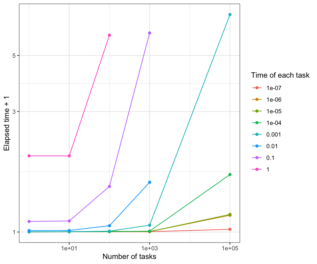
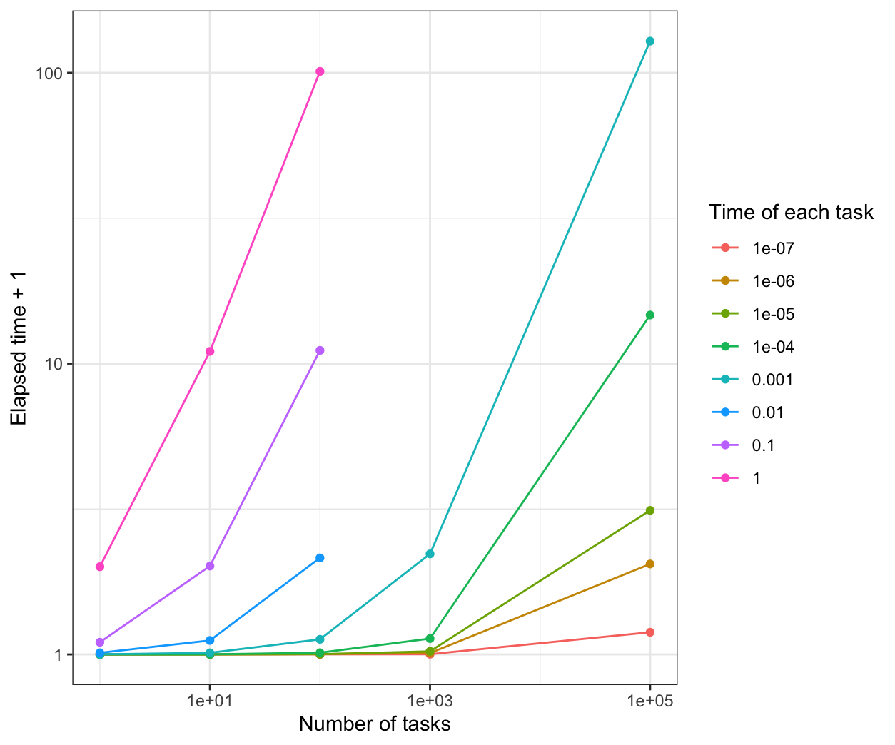
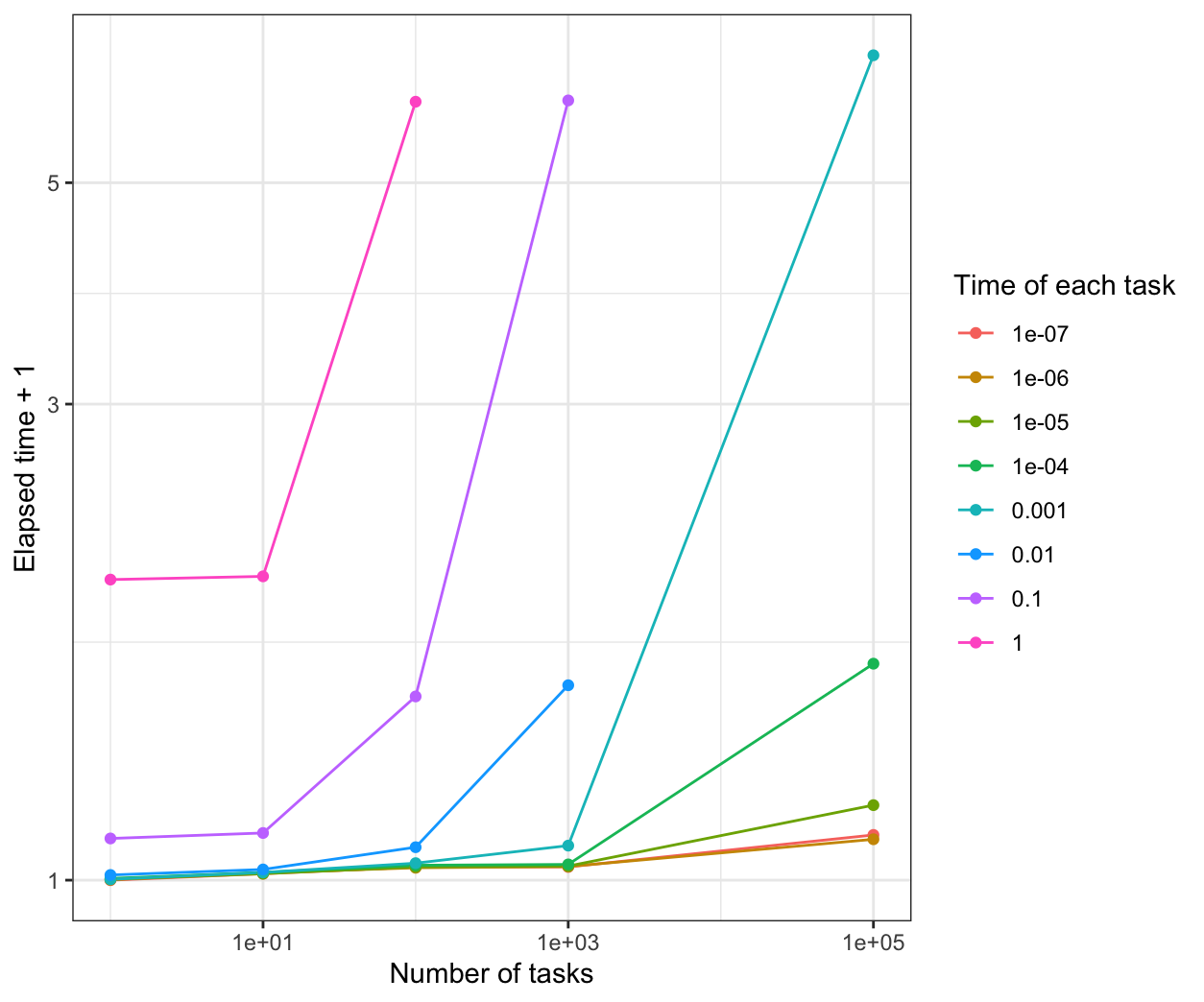
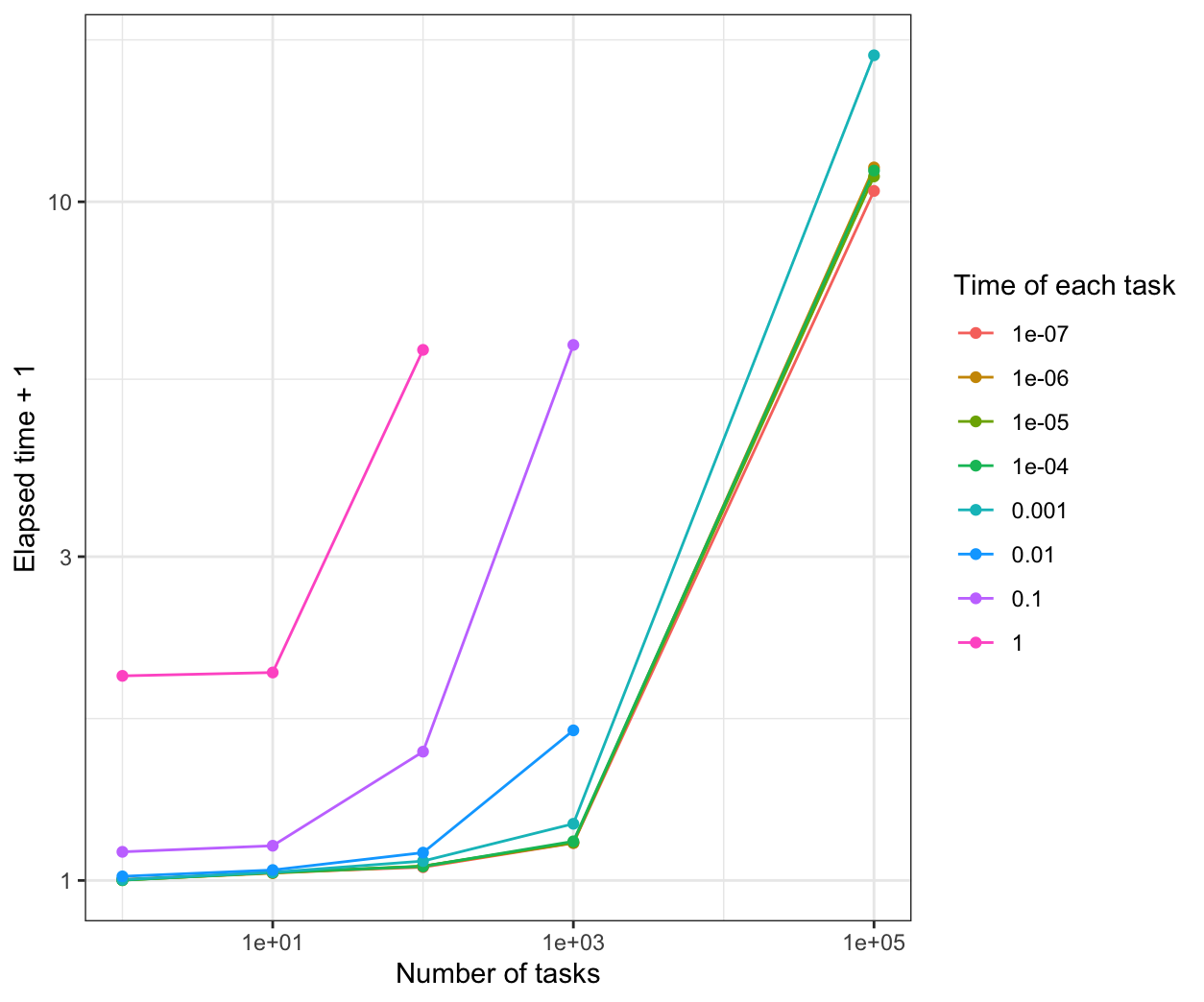
We compare all the results in the same plot:
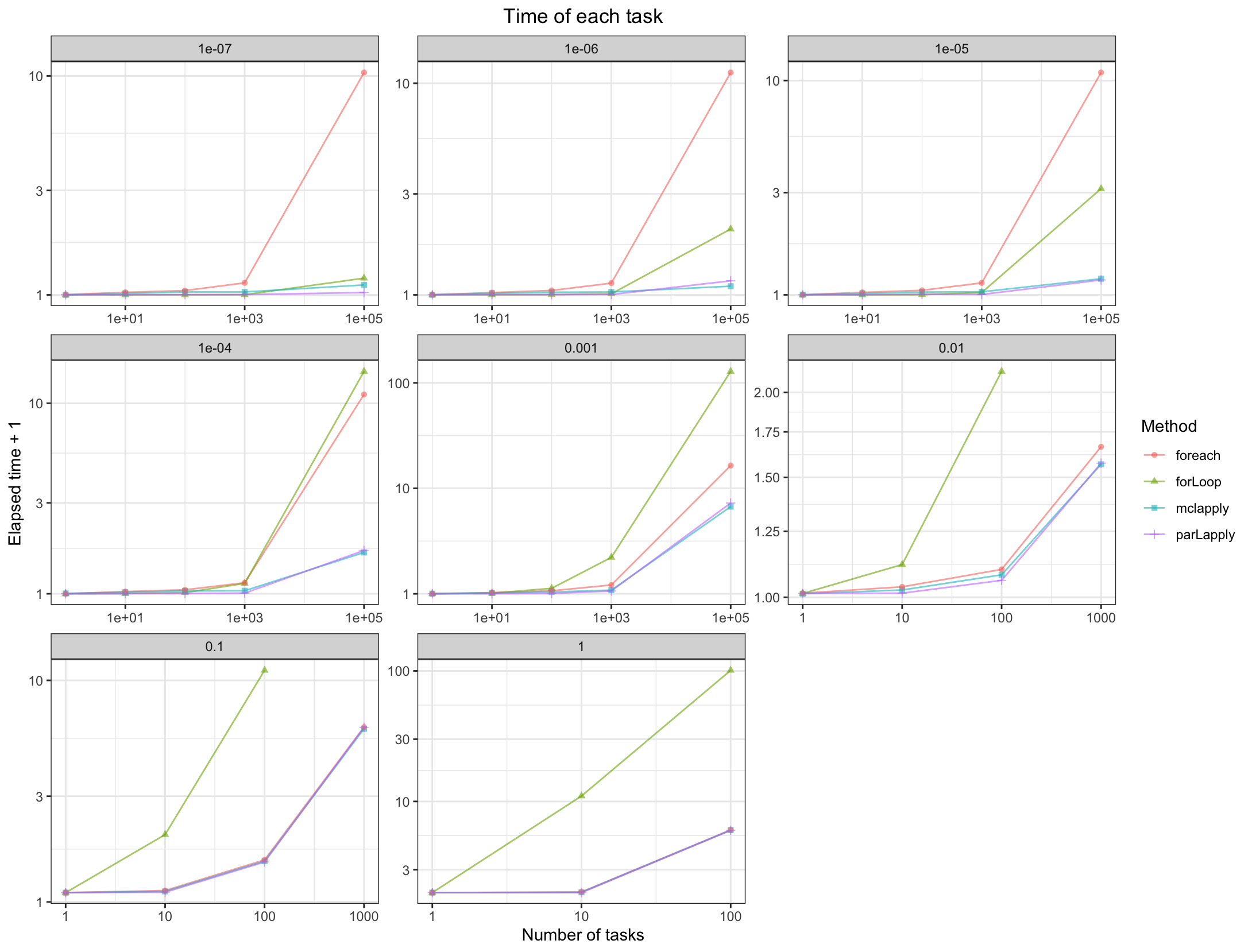
From the results, when the time of each task is more than 0.1s, all of the parallel methods have a good performance than the normal for loop.
When the time of each task is 1e-7s, parLapply will be the fastest.
When the time of each task is 1e-6s, mclapply will be the fastest.
When the time of each task is between 1e-5s to 0.01s, parLapply and mclapply are faster.
When the time of each task is less than 1e-5s, foreach is not better than the normal for loop.s When the time of each task is more than 1e-5s, foreach is faster than the normal for loop, but a little slower than parLapply and mclapply.
However, the performance is based on the sleep time for the system. If the calculation is considered in the program, the results and the performance may be different.